A.1(B)·Algebra II·Foundations for FunctionsReadiness

Modeling Data with Functions

Fit functions to tables and scatterplots, then use the model to predict and make decisions.

Students use differences and nearby scatterplot points to choose reasonable models, extend quadratic patterns, and estimate when a target output occurs.

Lesson plan and worked examples by TEKSForge · not a TEA-issued lesson. Videos by independent educators.

Archived course: TEKS code and readiness label from TEA's 2013 Algebra II key. Algebra II is not one of Texas's current required STAAR EOC assessments, and this lesson does not change the Biology and Algebra I Study Plans.

Practice the released item Ask the tutor All Algebra II released practice50 minutes

Learn the concept

Choose a family

With equally spaced inputs, nearly constant first differences suggest a linear model. Nearly constant nonzero second differences suggest a quadratic model. A rise followed by a fall is consistent with a downward-opening parabola.

Continue changing differences

If first differences decrease by 6 each time, subtract 6 again to predict the next difference, then add that difference to the previous output. Approximate data produce approximate predictions.

Read a target from a scatterplot

Locate the target output on the vertical axis and move horizontally to the local trend, then down to the input axis. Interpolation stays inside the data interval; extrapolation extends beyond it and is less dependable.

Study released STAAR visuals

Use the original graphs, tables, and diagrams from released STAAR questions to practice reading labels, values, and relationships before answering the items below.

Archived released STAAR Algebra II EOC · 2013 · Item 50 · 1 point

Weekly defective parts per 10,000 produced. Points: week 1 about 255, week 2 about 215, week 4 about 155, week 7 about 95, week 9 about 70, week 10 about 60. The y-axis has a break below 50. — Defective Parts scatterplotOriginal visual from the released STAAR test.

Worked example

A ball has heights 20, 44, 60, and 68 meters at times 0, 1, 2, and 3 seconds. Continue the quadratic pattern to estimate its height at 5 seconds.

First differences are $24,16,8$ .
Second differences are $-8,-8$ , so the next first differences are 0 and $-8$ .
At 4 seconds the height is $68+0=68$ ; at 5 seconds it is $68-8=60$ .

The model predicts 60 meters at 5 seconds.

Watch the lesson

Texas public-school, Texas educator-created, and TEKS-aligned lessons, hosted by their creators. Each card names its source.

Texas public school video

Algebra 2 Connecting Standard Form to Vertex Form

UT IPSI · Kid2Kid / Texas Education Agency

Connect a quadratic model’s turning point and changing rate to its graph.

Watch on YouTube

Try it yourself

TEKSForge practice · unscored

1. A trend passes near $(2,180)$ and $(6,100)$ . At what input is the output about 140?
Show answer and reasoning
$x\approx4$
The local slope is $(100-180)/(6-2)=-20$ . A drop of 40 takes about 2 input units after 2.
2. At inputs 0, 1, 2, 3 a table gives 7, 18, 25, 28. Predict the output at 4.
Show answer and reasoning
27
Differences are 11, 7, 3; the constant second difference is $-4$ . The next difference is $-1$ , so $28-1=27$ .

Released STAAR practice

Texas Education Agency · archived 2013 released EOC items · scored with TEA's answer key; step-by-step explanations written by TEKSForge because this release has no rationales. Original graphs, tables, and diagrams are shown where the released item includes one.

Archived released STAAR Algebra II EOC · 2013 · Item 15 · 1 point

An object is launched into the air. The table shows the object's height above the ground at various times. Based on the data in the table, which of the following is closest to the object's height above the ground 9 seconds after being launched?

Height vs. Time
Elapsed Time (seconds)	Height Above the Ground (meters)
1	78
2	109
3	131
4	143
5	145
6	137

110 m
55 m
10 m
95 m

Show STAAR answer and explanation

55 m

The heights rise and then fall, and the first differences (31, 22, 12, 2, −8) decrease by about 10 each second, so a quadratic model fits. Continuing the pattern gives differences of about −18, −28, and −38: $137-18=119$ at 7 s, $119-28=91$ at 8 s, and $91-38=53$ at 9 s, closest to 55 m.

110 m: 110 m is closer to the height at about 7.5 seconds; the object is falling faster each second after its peak.

10 m: Reaching 10 m would take another second or more of falling; continuing the differences gives about 53 m at 9 seconds.

95 m: Using a constant drop of 8 m per second ignores that the differences keep decreasing; the height falls faster after the peak.

Ask the tutor about this question

Archived released STAAR Algebra II EOC · 2013 · Item 50 · 1 point

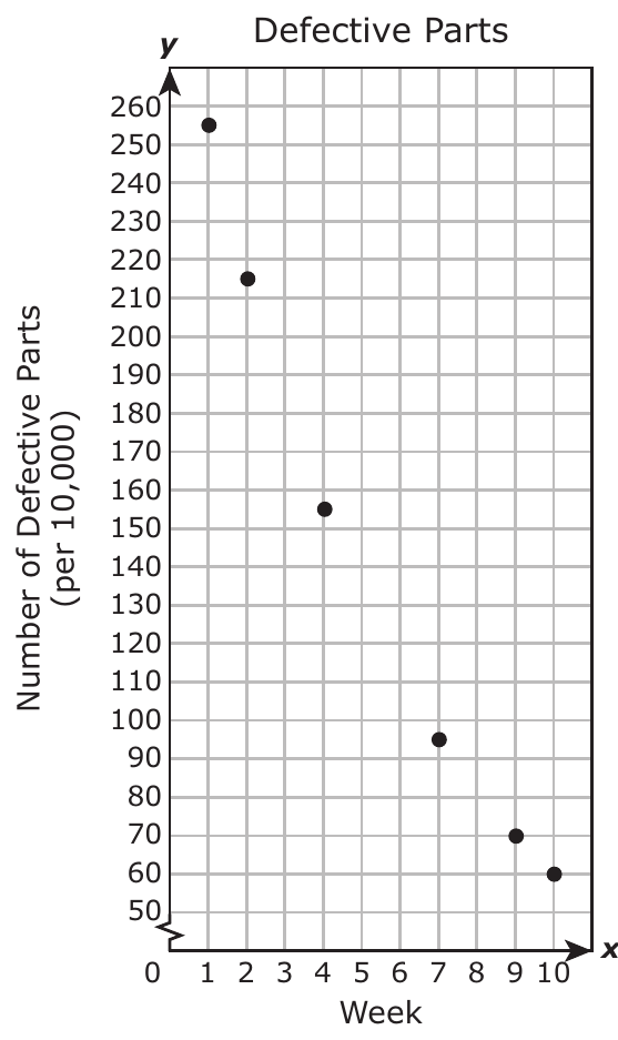
A factory began producing new parts. Data were collected on the number of defective parts per 10,000 parts produced. The graph shown displays some of the data for the first 10 weeks of production. Based on the graph, during which week were approximately 130 defective parts per 10,000 produced?

Week 3
Week 5
Week 6
Week 8

Show STAAR answer and explanation

Week 5

The points fall from 155 at week 4 to 95 at week 7, about 20 per week. Week 5 is about $155-20=135$ , closest to 130.

Week 3: Week 3 lies between 215 (week 2) and 155 (week 4), so it is about 185.

Week 6: Week 6 is about $155-2(20)=115$ .

Week 8: Week 8 lies between 95 (week 7) and 70 (week 9), so it is about 82.

Ask the tutor about this question

Start scored STAAR practice

Learning objectives

By the end of the lesson, students can:

Use first and second differences to distinguish linear and quadratic models.
Predict a value by extending a quadratic pattern.
Estimate an input from a scatterplot trend and discuss uncertainty.

Instructional sequence

1
Engage
5 min
Compare a straight trend with a rise-and-fall trend.
2
Direct instruction
10 min
Build first- and second-difference rows for equally spaced inputs.
3
Guided practice
13 min
Extend a quadratic height table beyond its last recorded time.
4
Compare and verify
15 min
Use nearby scatterplot points to estimate when a target value occurs.
5
Closure
7 min
Justify a model and complete the exit ticket.

Misconceptions to address

“Use the last first difference forever.”

Teacher move: A quadratic has changing first differences; continue the second-difference pattern.

“A fitted model gives an exact future measurement.”

Teacher move: Predictions are estimates, especially beyond the measured interval.

Materials

•Height-time tables
•Scatterplots with labeled scales
•Graphing calculator

Teaching tips

Check equal spacing of inputs before using differences.
Keep units in every prediction.
Ask whether a target calls for an input or an output.

Exit ticket · 3–5 min

For inputs 0, 1, 2, 3, outputs are 12, 22, 28, 30. Predict the output at 4.

Show expected answer

First differences are 10, 6, 2; the next is $-2$ , so the prediction is 28.

Sources & alignment

TEA 2013 Algebra II released test TEA 2013 Algebra II answer key and standards Texas Gateway, home of the UT IPSI Kid2Kid lessons

Alignment follows the standard TEA assigned to each 2013 released item. Video playback depends on YouTube access; written instruction remains available here.

Learn the concept

Choose a family

Continue changing differences

Read a target from a scatterplot

Study released STAAR visuals

Archived released STAAR Algebra II EOC · 2013 · Item 50 · 1 point

Worked example

Watch the lesson

Algebra 2 Connecting Standard Form to Vertex Form

Try it yourself

1. A trend passes near (2,180)(2,180)(2,180) and (6,100)(6,100)(6,100). At what input is the output about 140?

2. At inputs 0, 1, 2, 3 a table gives 7, 18, 25, 28. Predict the output at 4.

Released STAAR practice

Archived released STAAR Algebra II EOC · 2013 · Item 15 · 1 point

Archived released STAAR Algebra II EOC · 2013 · Item 50 · 1 point

Learning objectives

Instructional sequence

Engage

Direct instruction

Guided practice

Compare and verify

Closure

Misconceptions to address

1. A trend passes near $(2,180)$ and $(6,100)$ . At what input is the output about 140?